Give a session on C++ AMP – here is how

Wed, September 21, 2011, 06:53 PM under GPGPU | ParallelComputing

2/29/2012 added some Beta notes inline

Ever since presenting on C++ AMP at the AMD Fusion conference in June, then the Gamefest conference in August, and the BUILD conference in September, I've had numerous requests about my material from folks that want to re-deliver the same session. The C++ AMP session I put together has evolved over the 3 presentations to its final form that I used at BUILD, so that is the one I recommend you base yours on.BUILD session

Please get the slides and the recording from channel9 (I'll refer to slide numbers below).

This is how I've been presenting the C++ AMP session:

Context

  1. (slide 3, 04:18-08:18) Start with a demo, on my dual-GPU machine. I've been using the N-Body sample.
  2. (slide 4) Use an nvidia slide that has additional examples of performance improvements that customers enjoy with heterogeneous computing.
  3. (slide 5) Talk a bit about the differences today between CPU and GPU hardware, leading to the fact that these will continue to co-exist and that GPUs are great for data parallel algorithms, but not much else today. One is a jack of all trades and the other is a number cruncher.
  4. (slide 6) Use the APU example from amd, as one indication that the hardware space is still in motion, emphasizing that the C++ AMP solution is a data parallel API, not a GPU API. It has a future proof design for hardware we have yet to see.
  5. (slide 7) Provide more meta-data, as blogged about when I first introduced C++ AMP.

Code

  1. (slide 9-11) Introduce C++ AMP coding with a simplistic array-addition algorithm – the slides speak for themselves.
  2. (slide 12-13) index, and extent (Beta note: the old slide also refers to a grid class, which we removed in favor of just extent)
  3. (Slide 14-16) array, array_view and comparison between them.
  4. (Slide 17) parallel_for_each.
  5. (slide 18, 21) restrict.
  6. (slide 19-20) actual restrictions of restrict(amp) – the slides speak for themselves. (Beta note: the slide refers  to restrict(direct3d), which is now restrict(amp))
  7. (slide 22) bring it altogether with a matrix multiplication example.
  8. (slide 23-24) accelerator, and accelerator_view.
  9. (slide 26-29) Introduce tiling incl. tiled matrix multiplication [tiling probably deserves a whole session instead of 6 minutes!].

IDE

  1. (slide 34,37) Briefly touch on the concurrency visualizer. It supports GPU profiling, but enhancements specific to C++ AMP come at the Beta timeframe.
  2. (slide 35-36, 51:54-59:16) Demonstrate the GPU debugging experience in VS 11.

Summary

  1. (slide 39) Re-iterate some of the points of slide 7, and add the point that C++ AMP is an open specification.
  2. (slide 40) Links to content – see slide – including where all your questions should go: http://social.msdn.microsoft.com/Forums/en/parallelcppnative/threads.

Slides for similar presentation updated for Beta

The BUILD recording and slides are valid for the VS 11 Beta and beyond, with regards to C++ AMP - so watch the session and download those slides. Additionally, if you are going to repeat the session, I have updated the slides including some tweaks and you can download the updated deck here (note the slide numbers above do not map exactly to the new deck).

"But I don't have time for a full blown session, I only need 2 (or just 1, or 3) C++ AMP slides to use in my session on related topic X"

If all you want is a small number of slides, you can take some from the session above and customize them. But because I am so nice, I have created some slides for you, including talking points in the notes section. Download them here.


GPU Debugging with VS 11

Tue, September 20, 2011, 07:21 PM under GPGPU | ParallelComputing | VisualStudio

BELOW IS OUTDATED INFORMATION, PLEASE SEE MY UPDATED POST ON OUR TEAM BLOG:

http://blogs.msdn.com/b/nativeconcurrency/archive/2012/03/17/start-gpu-debugging-in-visual-studio-11.aspx

---

With VS 11 Developer Preview we have invested tremendously in parallel debugging for both CPU (managed and native) and GPU debugging. I'll be doing a whole bunch of blog posts on those topics, and in this post I just wanted to get people started with GPU debugging, i.e. with debugging C++ AMP code.

First I invite you to watch 6 minutes of a glimpse of the C++ AMP debugging experience though this video (ffw to minute 51:54, up until minute 59:16). Don't read the rest of this post, just go watch that video, ideally download the High Quality WMV.

Summary

GPU debugging essentially means debugging the lambda that you pass to the parallel_for_each call (plus any functions you call from the lambda, of course). CPU debugging means debugging all the code above and below the parallel_for_each call, i.e. all the code except the restrict(direct3d) lambda and the functions that it calls. With VS 11 you have to choose what debugger you want to use for a particular debugging session, CPU or GPU. So you can place breakpoints all over your code, then choose what debugger you want (CPU or GPU), and you'll only be able to hit breakpoints for the code type that the debugger engine understands – the remaining breakpoints will appear as unbound. If you want to hit the unbound breakpoints, you'd have to stop debugging, and start again with the other debugger. Sorry. We suck. We know. But once you are past that limitation, I think you'll find the experience truly rewarding – seriously!

Switching debugger engines

With the Developer Preview bits, one way to switch the debugger engine is through the project properties – see the screenshots that follow.

This one is showing the CPU option selected, which is basically the default that you are all familiar with:

image

This screenshot is showing the GPU option selected, by changing the debugger launcher (notice that this applies for both the local and remote case):

image

You actually do not have to open the project properties just for switching the debugger engine, you can switch the selection from the toolbar in VS 11 Developer Preview too – see following screenshot (the effect is the same as if you opened the project properties and switched there)

image

Breakpoint behavior

Here are two screenshots, one showing a debugging session for CPU and the other a debugging session for GPU (notice the unbound breakpoints in each case)

image

…and here is the GPU case (where we cannot bind the CPU breakpoints but can the GPU breakpoint, which is actually hit)

image

Give C++ AMP debugging a try

So to debug your C++ AMP code, pull down the drop down under the 'play' button to select the 'GPU C++ Direct3D Compute Debugger' menu option, then hit F5 (or the 'play' button itself). Then you can explore debugging by exploring the menus under the Debug and under the Debug->Windows menus. One way to do that exploration is through the C++ AMP debugging walkthrough on MSDN.

Another way to explore the C++ AMP debugging experience, you can use the moth.cpp code file, which is what I used in my BUILD session debugger demo. Note that for my demo I was using the latest internal VS11 bits, so your experience with the Developer Preview bits won't be identical to what you saw me demonstrate, but it shouldn't be far off.

Stay tuned for a lot more content on the parallel debugger in VS 11, both CPU and GPU, both managed and native.


Running C++ AMP kernels on the CPU

Mon, September 19, 2011, 07:32 PM under GPGPU | ParallelComputing

One of the FAQs we receive is whether C++ AMP can be used to target the CPU.

For targeting multi-core we have a technology we released with VS2010 called PPL, which has had enhancements for VS 11 – that is what you should be using! FYI, it also has a Linux implementation via Intel's TBB which conforms to the same interface.

When you choose to use C++ AMP, you choose to take advantage of massively parallel hardware, through accelerators like the GPU.

Having said that, you can always use the accelerator class to check if you are running on a system where the is no hardware with a DirectX 11 driver, and decide what alternative code path you wish to follow. 

In fact, if you do nothing in code, if the runtime does not find DX11 hardware to run your code on, it will choose the WARP accelerator which will run your code on the CPU, taking advantage of multi-core and SSE2 (depending on the CPU capabilities WARP also uses SSE3 and SSE 4.1 – it does not currently use AVX and on such systems you hopefully have a DX 11 GPU anyway).

A few things to know about WARP

  • It is our fallback CPU solution, not intended as a primary target of C++ AMP.
  • WARP stands for Windows Advanced Rasterization Platform and you can read old info on this MSDN page on WARP.
  • What is new in Windows 8 Developer Preview is that WARP now supports DirectCompute, which is what C++ AMP builds on.
  • It is not currently clear if we will have a CPU fallback solution for non-Windows 8 platforms when we ship.
  • When you create a WARP accelerator, its is_emulated property returns true.
  • WARP does not currently support double precision.


BTW, when we refer to WARP, we refer to this accelerator described above. If we use lower case "warp", that refers to a bunch of threads that run concurrently in lock step and share the same instruction. In the VS 11 Developer Preview, the size of warp in our Ref emulator is 4 – Ref is another emulator that runs on the CPU, but it is extremely slow not intended for production, just for debugging.


Links to C++ AMP and other content

Fri, September 16, 2011, 10:00 PM under GPGPU | Links | ParallelComputing | VisualStudio | Windows

A few links you may be interested in.


BUILD apps that use C++ AMP

Tue, September 13, 2011, 08:28 PM under Events | GPGPU | ParallelComputing

If you are a developer on the Microsoft platform, you are hopefully attending (live or virtually) the sessions of the BUILD conference, aka //build/ in Anaheim, CA. The conference sold out not long after it opened registration, and it achieved that without sharing *any* session details nor a meaningful agenda up until after the keynote today – impressive!

I am speaking at BUILD and hope you'll catch my talk at 9am on Friday (the last day of the conference) at Marriott Elite 2 Ballroom. Session details follow.

802 - Taming GPU compute with C++ AMP

Developers today inject parallelism into their compute-intensive applications in order to take advantage of multi-core CPU hardware. Beyond CPUs, however, compute accelerators such as general-purpose GPUs can provide orders of magnitude speed-ups for data parallel algorithms. How can you as a C++ developer fully utilize this heterogeneous hardware from your Visual Studio environment?  How can you benefit from this tremendous performance boost in your Visual C++ solutions without sacrificing developer productivity?  The answers will be presented in this session about C++ Accelerated Massive Parallelism.

I'll be covering a lot of the material I've been recently blogging about on my blog that you are reading, which I have also indexed over on our team blog under the title: "C++ AMP in a nutshell".


tile_static, tile_barrier, and tiled matrix multiplication with C++ AMP

Sun, September 11, 2011, 06:23 PM under GPGPU | ParallelComputing

We ended the previous post with a mechanical transformation of the C++ AMP matrix multiplication example to the tiled model and in the process introduced tiled_index and tiled_extent. This is part 2.

tile_static memory

You all know that in regular CPU code, static variables have the same value regardless of which thread accesses the static variable. This is in contrast with non-static local variables, where each thread has its own copy.

Back to C++ AMP, the same rules apply and each thread has its own value for local variables in your lambda, whereas all threads see the same global memory, which is the data they have access to via the array and array_view.

In addition, on an accelerator like the GPU, there is a programmable cache, a third kind of memory type if you'd like to think of it that way (some call it shared memory, others call it scratchpad memory). Variables stored in that memory share the same value for every thread in the same tile. So, when you use the tiled model, you can have variables where each thread in the same tile sees the same value for that variable, that threads from other tiles do not. The new storage class for local variables introduced for this purpose is called tile_static. You can only use tile_static in restrict(amp) functions, and only when explicitly using the tiled model. What this looks like in code should be no surprise, but here is a snippet to confirm your mental image, using a good old regular C array

  // each tile of threads has its own copy of locA,
  // shared among the threads of the tile
  tile_static float locA[16][16]; 

Note that tile_static variables are scoped and have the lifetime of the tile, and they cannot have constructors or destructors.

tile_barrier

In amp.h one of the types introduced is tile_barrier. imageYou cannot construct this object yourself (although if you had one, you could use a copy constructor to create another one). So how do you get one of these? You get it, from a tiled_index object. Beyond the 4 properties returning index objects, tiled_index has another property, barrier, that returns a tile_barrier object. The tile_barrier class exposes the method wait (and other wait overloads).

15:  // Given a tiled_index object named t_idx
16:  t_idx.barrier.wait();

17:  // more code

…in the code above, all threads in the tile will reach line 16 before a single one progresses to line 17. Note that all threads must be able to reach the barrier, i.e. if you had branchy code in such a way which meant that there is a chance that not all threads could reach line 16, then the code above would be illegal.

Tiled Matrix Multiplication Example – part 2

So now that we added to our understanding the concepts of tile_static and tile_barrier, let me obfuscate rewrite the matrix multiplication code so that it takes advantage of tile_static memory. Before you start reading this, I suggest you get a cup of your favorite non-alcoholic beverage to enjoy while you try to fully understand the code.

01: void MatrixMultiplyTiled(vector<float>& vC, 
         const vector<float>& vA, 
         const vector<float>& vB, int M, int N, int W)
02: {
03:   static const int TS = 16;

04:   array_view<const float,2> a(M, W, vA);
05:   array_view<const float,2> b(W, N, vB);
06:   array_view<float,2> c(M,N,vC); c.discard_data();

07:   parallel_for_each(c.extent.tile< TS, TS >(),
08:   [=] (tiled_index< TS, TS> t_idx) restrict(amp) 
09:   {
10:     int row = t_idx.local[0]; int col = t_idx.local[1];
11:     float sum = 0.0f;

12:     for (int i = 0; i < W; i += TS) {
13:        tile_static float locA[TS][TS], locB[TS][TS];
14:        locA[row][col] = a(t_idx.global[0], col + i);
15:        locB[row][col] = b(row + i, t_idx.global[1]);
16:        t_idx.barrier.wait();

17:        for (int k = 0; k < TS; k++)
18:          sum += locA[row][k] * locB[k][col];

19:        t_idx.barrier.wait();
20:     }

21:     c[t_idx.global] = sum;
22:   });
23: }

Notice that all the code up to line 9 is the same as per the changes we made in part 1 of tiling introduction. If you squint, the body of the lambda itself preserves the original algorithm on lines 10, 11, and 17, 18, and 21. The difference being that those lines use new indexing and the tile_static arrays; the tile_static arrays are declared and initialized on the brand new lines 13-15. On those lines we copy from the global memory represented by the array_view objects (a and b), to the tile_static vanilla arrays (locA and locB)we are copying enough to fit a tile. Because in the code that follows on line 18 we expect the data for this tile to be in the tile_static storage, we need to synchronize the threads within each tile with a barrier, which we do on line 16 (to avoid accessing uninitialized memory on line 18). We also need to synchronize the threads within a tile on line 19, again to avoid the race between lines 14, 15 (retrieving the next set of data for each tile and overwriting the previous set) and line 18 (not being done processing the previous set of data). Luckily, as part of the awesome C++ AMP debugger in Visual Studio there is an option that helps you find such races, but that is a story for another blog post another time.

May I suggest reading the next section, and then coming back to re-read and walk through this code with pen and paper to really grok what is going on, if you haven't already? Cool.

Why would I introduce this tiling complexity into my code?

Funny you should ask that, I was just about to tell you. There is only one reason we tiled our extent, had to deal with finding a good tile size, ensure the number of threads we schedule are correctly divisible with the tile size, had to use a tiled_index instead of a normal index, and had to understand tile_barrier and to figure out where we need to use it, and double the size of our lambda in terms of lines of code: the reason is to be able to use tile_static memory.

Why do we want to use tile_static memory? Because accessing tile_static memory is around 10 times faster than accessing the global memory on an accelerator like the GPU, e.g. in the code above, if you can get 150GB/second accessing data from the array_view a, you can get 1500GB/second accessing the tile_static array locA. And since by definition you are dealing with really large data sets, the savings really pay off. We have seen tiled implementations being twice as fast as their non-tiled counterparts.

Now, some algorithms will not have performance benefits from tiling (and in fact may deteriorate), e.g. algorithms that require you to go only once to global memory may not benefit from tiling, since with tiling you already have to fetch the data once from global memory! Other algorithms may benefit, but you may decide that you are happy with your code being 50 times faster than the serial-version you had, and you do not need to invest to make it 100 times faster. Also algorithms with more than 3 dimensions, which C++ AMP supports in the simple model, cannot be tiled.

Also note that in future releases, we may invest in making the non-tiled model, which already uses tiling under the covers, go the extra step and use tile_static memory on your behalf, but it is obviously way to early to commit to anything like that, and we certainly don't do any of that today.


Scheduling thread tiles with C++ AMP

Sat, September 10, 2011, 08:30 PM under GPGPU | ParallelComputing

This post assumes you are totally comfortable with, what some of us call, the simple model of C++ AMP, i.e. you could write your own matrix multiplication. We are now ready to explore the tiled model, which builds on top of the non-tiled one.

Tiling the extent

We know that when we pass an extent to the parallel_for_each call, it determines the number of threads to schedule and their index values (including dimensionality). For the single-, two-, and three- dimensional cases you can go a step further and subdivide the threads into what we call tiles of threads (others may call them thread groups).

So here is a single-dimensional example:

  extent<1> e(20);   // 20 units in a single dimension with indices from 0-19
  tiled_extent<4> te = e.tile<4>();

…on the 2nd line we subdivided the single-dimensional space into 5 single-dimensional tiles each having 4 elements, and we captured that result in a concurrency::tiled_extent (a new class in amp.h).

Let's move on swiftly to another example, in pictures, this time 2-dimensional:

image

So we start on the left with a 2-dimensional extent which has 8*6=48 threads. We then have two different examples of tiling. In the first case, in the middle, we subdivide the 48 threads into tiles where each has 4*3=12 threads, hence we have 2*2=4 tiles. In the second example, on the right, we subdivide the original input into tiles where each has 2*2=4 threads, hence we have 4*3=12 tiles. Notice how you can play with the tile size and achieve different number of tiles. The numbers you pick must be such that the original total number of threads (in our example 48), remains the same, and every tile must have the same size.

Of course, you still have no clue why you would do that, but stick with me. First, we should see how we can use this tiled_extent, since the parallel_for_each function that we know expects a extent.

Tiled parallel_for_each and tiled_index

It turns out that we have additional overloads of parallel_for_each that accept a tiled_extent instead of a extent. However, those overloads, also expect that the lambda you pass in accepts a concurrency::tiled_index (new in amp.h), not an index<N>. So how is a tiled_index different to an index?

A tiled_index object, can have only 1 or 2 or 3 dimensions (matching exactly the tiled_extent), and consists of 4 index objects that are accessible via properties: global, local, tile_origin, and tile. The global index is the same as the index we know and love: the global thread ID. The local index is the local thread ID within the tile. The tile_origin index returns the global index of the thread that is at position 0,0 of this tile, and the tile index is the position of the tile in relation to the overall grid. Confused? Here is an example accompanied by a picture that hopefully clarifies things:image

  array_view<int, 2> data(8, 6, p_my_data);
  parallel_for_each(data.extent.tile<2,2>(), [=](tiled_index<2,2> t_idx) restrict(amp) { ... });

Given the code above and the picture on the right, what are the values of each of the 4 index objects that the t_idx variables exposes, when the lambda is executed by T (highlighted in the picture on the right)?

If you can't work it out yourselves, the solution follows:

  • t_idx.global       = index<2> (6,3)
  • t_idx.local          = index<2> (0,1)
  • t_idx.tile_origin = index<2> (6,2)
  • t_idx.tile             = index<2> (3,1)

Don't move on until you are comfortable with this… the picture really helps, so use it.

Tiled Matrix Multiplication Example – part 1

Let's paste here the C++ AMP matrix multiplication example, bolding the lines we are going to change (can you guess what the changes will be?)

01:  void MatrixMultiplyTiled_Part1(vector<float>& vC, 
         const vector<float>& vA, 
         const vector<float>& vB, int M, int N, int W)
02:  {
03:
04:    array_view<const float,2> a(M, W, vA);
05:    array_view<const float,2> b(W, N, vB);
06:    array_view<float,2> c(M, N, vC); c.discard_data();

07:    parallel_for_each(c.extent, 
08:    [=](index<2> idx) restrict(amp) {
09:
10:      int row = idx[0]; int col = idx[1];
11:      float sum = 0.0f;
12:      for(int i = 0; i < W; i++)
13:        sum += a(row, i) * b(i, col);
14:      c[idx] = sum;
15:    });
16:  }

To turn this into a tiled example, first we need to decide our tile size. Let's say we want each tile to be 16*16 (which assumes that we'll have at least 256 threads to process, and that c.extent.size() is divisible by 256, and moreover that c.extent[0] and c.extent[1] are divisible by 16). So we insert at line 03 the tile size (which must be a compile time constant).

03: static const int TS = 16;

...then we need to tile the extent to have tiles where each one has 16*16 threads, so we change line 07 to be as follows

07: parallel_for_each(c.extent.tile<TS,TS>(),

...that means that our index now has to be a tiled_index with the same characteristics as the tiled_extent, so we change line 08

08: [=](tiled_index<TS, TS> t_idx) restrict(amp) {

...which means, without changing our core algorithm, we need to be using the global index that the tiled_index gives us access to, so we insert line 09 as follows

09: index<2> idx = t_idx.global;

...and now this code just works and it is tiled!

Closing thoughts on part 1

The process we followed just shows the mechanical transformation that can take place from the simple model to the tiled model (think of this as step 1). In fact, when we wrote the matrix multiplication example originally, the compiler was doing this mechanical transformation under the covers for us (and it has additional smarts to deal with the cases where the total number of threads scheduled is not divisible by the tile size). The point is that the thread scheduling is always tiled, even when you use the non-explicitly-tiled model.

But with this mechanical transformation, we haven't gained anything… Hint: our goal with explicitly using the tiled model is to gain even more performance.

In the next post, we'll evolve this further (beyond what the compiler can automatically do for us, in this first release), so you can see the full usage of the tiled model and its benefits…


Matrix Multiplication with C++ AMP

Fri, September 9, 2011, 08:22 PM under GPGPU | ParallelComputing

As part of our API tour of C++ AMP, we looked recently at parallel_for_each. I ended that post by saying we would revisit parallel_for_each after introducing array and array_view. Now is the time, so this is part 2 of parallel_for_each, and also a post that brings together everything we've seen until now.

The code for serial and accelerated

Consider a naïve (or brute force) serial implementation of matrix multiplication 

0:  void MatrixMultiplySerial(std::vector<float>& vC, 
        const std::vector<float>& vA, 
        const std::vector<float>& vB, int M, int N, int W)
1:  {
2:    for (int row = 0; row < M; row++) 
3:    {
4:      for (int col = 0; col < N; col++)
5:      {
6:        float sum = 0.0f;
7:        for(int i = 0; i < W; i++)
8:          sum += vA[row * W + i] * vB[i * N + col];
9:        vC[row * N + col] = sum;
10:     }
11:   }
12: }

We notice that each loop iteration is independent from each other and so can be parallelized. If in addition we have really large amounts of data, then this is a good candidate to offload to an accelerator. First, I'll just show you an example of what that code may look like with C++ AMP, and then we'll analyze it. It is assumed that you included at the top of your file #include <amp.h>

13:  void MatrixMultiplySimple(std::vector<float>& vC, 
         const std::vector<float>& vA, 
         const std::vector<float>& vB, int M, int N, int W)
14:  {
15:    concurrency::array_view<const float,2> a(M, W, vA);
16:    concurrency::array_view<const float,2> b(W, N, vB);
17:    concurrency::array_view<float,2> c(M, N, vC); c.discard_data();
18:    concurrency::parallel_for_each(c.extent, 
19:    [=](concurrency::index<2> idx) restrict(amp) {
20:      int row = idx[0]; int col = idx[1];
21:      float sum = 0.0f;
22:      for(int i = 0; i < W; i++)
23:        sum += a(row, i) * b(i, col);
24:      c[idx] = sum;
25:    });
26:  }

First a visual comparison, just for fun: The beginning and end is the same, i.e. lines 0,1,12 are identical to lines 13,14,26. The double nested loop (lines 2,3,4,5 and 10,11) has beenMatrix Multiplication image from wikipedia transformed into a parallel_for_each call (18,19,20 and 25). The core algorithm (lines 6,7,8,9) is essentially the same (lines 21,22,23,24). We have extra lines in the C++ AMP version (15,16,17). Now let's dig in deeper.

Using array_view and extent

When we decided to convert this function to run on an accelerator, we knew we couldn't use the std::vector objects in the restrict(amp) function. So we had a choice of copying the data to the the concurrency::array<T,N> object, or wrapping the vector container (and hence its data) with a concurrency::array_view<T,N> object from amp.h – here we used the latter (lines 15,16,17). Now we can access the same data through the array_view objects (a and b) instead of the vector objects (vA and vB), and the added benefit is that we can capture the array_view objects in the lambda (lines 19-25) that we pass to the parallel_for_each call (line 18) and the data will get copied on demand for us to the accelerator.

Note that line 15 (and ditto for 16 and 17) could have been written as two lines instead of one:

  extent<2> e(M, W);
  array_view<const float, 2> a(e, vA);

In other words, we could have explicitly created the extent object instead of letting the array_view create it for us under the covers through the constructor overload we chose. The benefit of the extent object in this instance is that we can express that the data is indeed two dimensional, i.e a matrix. When we were using a vector object we could not do that, and instead we had to track via additional unrelated variables the dimensions of the matrix (i.e. with the integers M and W) – aren't you loving C++ AMP already?

Note that the const before the float when creating a and b, will result in the underling data only being copied to the accelerator and not be copied back – a nice optimization. A similar thing is happening on line 17 when creating array_view c, where we have indicated that we do not need to copy the data to the accelerator, through the discard_data call.

The kernel dispatch

On line 18 we make the call to the C++ AMP entry point (parallel_for_each) to invoke our parallel loop or, as some may say, dispatch our kernel.

The first argument we need to pass describes how many threads we want for this computation. For this algorithm we decided that we want exactly the same number of threads as the number of elements in the output matrix, i.e. in array_view c which will eventually update the vector vC. So each thread will compute exactly one result. Since the elements in c are organized in a 2-dimensional manner we can organize our threads in a two-dimensional manner too. We don't have to think too much about how to create the first argument (a extent) since the array_view object helpfully exposes that as a property. Note that instead of c.extent we could have written extent<2>(M, N) – the result is the same in that we have specified M*N threads to execute our lambda.

The second argument is a restrict(amp) lambda that accepts an index object. Since we elected to use a two-dimensional extent as the first argument of parallel_for_each, the index will also be two-dimensional and as covered in the previous posts it represents the thread ID, which in our case maps perfectly to the index of each element in the resulting array_view.

The kernel itself

The lambda body (lines 20-24), or as some may say, the kernel, is the code that will actually execute on the accelerator. It will be called by M*N threads and we can use those threads to index into the two input array_views (a,b) and write results into the output array_view ( c ).

The four lines (21-24) are essentially identical to the four lines of the serial algorithm (6-9). The only difference is how we index into a,b,c versus how we index into vA,vB,vC. The code we wrote with C++ AMP is much nicer in its indexing, because the dimensionality is a first class concept, so you don't have to do funny arithmetic calculating the index of where the next row starts, which you have to do when working with vectors directly (since they store all the data in a flat manner).

I skipped over describing line 20. Note that we didn't really need to read the two components of the index into temporary local variables. This mostly reflects my personal choice, in some algorithms to break down the index into local variables with names that make sense for the algorithm, i.e. in this case row and col. In other cases it may i,j,k or x,y,z, or M,N or whatever. Also note that we could have written line 24 as: c(idx[0], idx[1])=sum  or  c(row, col)=sum instead of the simpler c[idx]=sum

Targeting a specific accelerator

Imagine that we had more than one hardware accelerator on a system and we wanted to pick a specific one to execute this parallel loop on. So there would be some code like this anywhere before line 18:

  vector<accelerator> accs = MyFunctionThatChoosesSuitableAccelerators();
  accelerator acc = accs[0];

…and then we would modify line 18 so we would be calling another overload of parallel_for_each that accepts an accelerator_view as the first argument, so it would become:

  concurrency::parallel_for_each(acc.default_view, c.extent,

...and the rest of your code remains the same… how simple is that?


array and array_view from amp.h

Thu, September 8, 2011, 12:02 AM under GPGPU | ParallelComputing

This is a very long post, but it also covers what are probably the classes (well, array_view at least) that you will use the most with C++ AMP, so I hope you enjoy it!

Overview

The concurrency::array and concurrency::array_view template classes represent multi-dimensional data of type T, of N dimensions, specified at compile time (and you can later access the number of dimensions via the rank property). If N is not specified, it is assumed that it is 1 (i.e. single-dimensional case). They are rectangular (not jagged).array
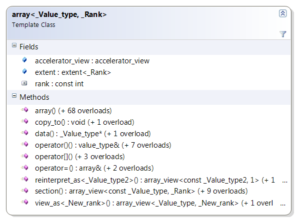
The difference between them is that array is a container of data, whereas array_view is a wrapper of a container of data. So in that respect, array behaves like an STL container, whereas the closest thing an array_view behaves like is an STL iterator (albeit with random access and allowing you to view more than one element at a time!).

The data in the array (whether provided at creation time or added later) resides on an accelerator (which is specified at creation time either explicitly by the developer, or set to the default accelerator at creation time by the runtime) and is laid out contiguously in memory. The data provided to the array_view is not stored by/in the array_view, because the array_view is simply a view over the real source (which can reside on the CPU or other accelerator). The underlying data is copied on demand to wherever the array_view is accessed. Elements which differ by one in the least significant dimension of the array_view are adjacent in memory.

array objects must be captured by reference into the lambda you pass to the parallel_for_each call, whereas array_view objects must be captured by value (into the lambda you pass to the parallel_for_each call). After you are done reading this post, feel free to visit another post dedicated to capturing data.

Creating array and array_view objects and relevant properties

You can create array_view objects from other array_view objects of the same rank and element type (shallow copy, also possible via assignment operator) so they point to the same underlying data, and you can also create array_view objects over array objects of the same rank and element type e.g.

  array_view<int,3> a(b); // b can be another array or array_view of ints with rank=3

Note: Unlike the constructors above which can be called anywhere, the ones in the rest of this section can only be called from CPU code.

You can create array objects from other array objects of the same rank and element type (copy and move constructors) and from other array_view objects, e.g.

  array<float,2> a(b); // b can be another array or array_view of floats with rank=2

To create an array from scratch, you need to at least specify an extent object, e.g. array<int,3> a(myExtent);. Note that instead of an explicit extent object, there are convenience overloads when N<=3 so you can specify 1-, 2-, 3- integers (dependent on the array's rank) and thus have the extent created for you under the covers. At any point, you can access the array's extent thought the extent property. The exact same thing applies to array_view (extent as constructor parameters, incl. convenience overloads, and property).

While passing only an extent object to create an array is enough (it means that the array will be written to later), it is not enough for the array_view case which must always wrap over some other container (on which it relies for storage space and actual content). So in addition to the extent object (that describes the shape you'd like to be viewing/accessing that data through), to create an array_view from another container (e.g. std::vector) you must pass in the container itself (which must expose .data() and a .size() methods, e.g. like std::array does), e.g.

  array_view<int,2> aaa(myExtent, myContainerOfInts);

Similarly, you can create an array_view from a raw pointer of data plus an extent object.

Back to the array case, to optionally initialize the array with data, you can pass an iterator pointing to the start (and optionally one pointing to the end of the source container) e.g.

  array<double,1> a(5, myVector.begin(), myVector.end());

We saw that arrays are bound to an accelerator at creation time, so in case you don’t want the C++ AMP runtime to assign the array to the default accelerator, all array constructors have overloads that let you pass an accelerator_view object, which you can later access via the accelerator_view property.

Note that at the point of initializing an array with data, a synchronous copy of the data takes place to the accelerator, and then to copy any data back we'll see that an explicit copy call is required. This does not happen with the array_view where copying is on demand...

refresh and synchronize on array_view

Note that in the previous section on constructors, unlike the array case, there was no overload that accepted an accelerator_view for array_view. That is because the array_view is simply a wrapper, so the allocation of the data has already taken place before you created the array_view. When you capture an array_view variable in your call to parallel_for_each, the copy of data between the non-CPU accelerator and the CPU takes place on demand (i.e. it is implicit, versus the explicit copy that has to happen with the array). There are some subtleties to the on-demand-copying that we cover next.array_view
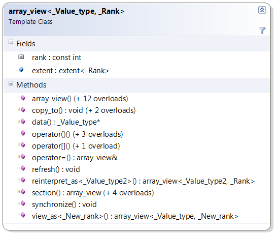
The assumption when using an array_view is that you will continue to access the data through the array_view, and not through the original underlying source, e.g. the pointer to the data that you passed to the array_view's constructor. So if you modify the data through the array_view on the GPU, the original pointer on the CPU will not "know" that, unless one of two things happen:

  • you access the data through the array_view on the CPU side, i.e. using indexing that we cover below
  • you explicitly call the array_view's synchronize method on the CPU (this also gets called in the array_view's destructor for you)

Conversely, if you make a change to the underlying data through the original source (e.g. the pointer), the array_view will not "know" about those changes, unless you call its refresh method.

Finally, note that if you create an array_view of const T, then the data is copied to the accelerator on demand, but it does not get copied back, e.g.

  array_view<const double, 5> myArrView(…); // myArrView will not get copied back from GPU

There is also a similar mechanism to achieve the reverse, i.e. not to copy the data of an array_view to the GPU.

copy_to, data, and global copy/copy_async functions

Both array and array_view expose two copy_to overloads that allow copying them to another array, or to another array_view, and these operations can also be achieved with assignment (via the = operator overloads).

Also both array and array_view expose a data method, to get a raw pointer to the underlying data of the array or array_view, e.g. float* f = myArr.data();. Note that for array_view, this only works when the rank is equal to 1, due to the data only being contiguous in one dimension as covered in the overview section.

Finally, there are a bunch of global concurrency::copy functions returning void (and corresponding concurrency::copy_async functions returning a future) that allow copying between arrays and array_views and iterators etc.

Note that for array, all copying described throughout this post is deep copying, as per other STL container expectations. You can never have two arrays point to the same data.

indexing into array and array_view plus projection

Reading or writing data elements of an array is only legal when the code executes on the same accelerator as where the array was bound to. In the array_view case, you can read/write on any accelerator, not just the one where the original data resides, and the data gets copied for you on demand. In both cases, the way you read and write individual elements is via indexing as described next.

To access (or set the value of) an element, you can index into it by passing it an index object via the subscript operator. Furthermore, if the rank is 3 or less, you can use the function ( ) operator to pass integer values instead of having to use an index object. e.g.

  array<float,2> arr(someExtent, someIterator); //or array_view<float,2> arr(someExtent, someContainer);
  index<2> idx(5,4);
  float f1 = arr[idx];
  float f2 = arr(5,4); //f2 ==f1
  //and the reverse for assigning, e.g.
  arr(idx[0], 7) = 6.9;

Note that for both array and array_view, regardless of rank, you can also pass a single integer to the subscript operator which results in a projection of the data, and (for both array and array_view) you get back an array_view of rank N-1 (or if the rank was 1, you get back just the element at that location).

Not Covered

In this already very long post, I am not going to cover three very cool methods (and related overloads) that both array and array_view expose: view_as, section, reinterpret_as. We'll revisit those at some point in the future, probably on the team blog.


parallel_for_each from amp.h – part 1

Tue, September 6, 2011, 07:52 PM under GPGPU | ParallelComputing

This posts assumes that you've read my other C++ AMP posts on index<N> and extent<N>, as well as about the restrict modifier. It also assumes you are familiar with C++ lambdas (if not, follow my links to C++ documentation).

Basic structure and parameters

Now we are ready for part 1 of the description of the new overload for the concurrency::parallel_for_each function. The basic new parallel_for_each method signature returns void and accepts two parameters:

  • a extent<N>
  • a restrict(amp) lambda, whose signature is such that it returns void and accepts an index of the same rank as the extent

So it looks something like this (with generous returns for more palatable formatting) assuming we are dealing with a 2-dimensional space:

  // some_code_A
  parallel_for_each(
    e, // e  is of type extent<2>
    [ ](index<2> idx) restrict(amp)
    {
      // kernel code
    }
  );
  // some_code_B

The parallel_for_each will execute the body of the lambda (which must have the restrict modifier), on the GPU. We also call the lambda body the "kernel". The kernel will be executed multiple times, once per scheduled GPU thread. The only difference in each execution is the value of the index object (aka as the GPU thread ID in this context) that gets passed to your kernel code. The number of GPU threads (and the values of each index) is determined by the extent object you pass, as described next.

In this context, one way to think about it is that the extent generates a number of index objects. So for the example above, if your extent was setup by some_code_A as follows:

  extent<2> e(2,3);

...then given that: e.size()==6, e[0]==2, and e[1]==3

...the six index<2> objects it generates (and hence the values that your lambda would receive) are:

   (0,0) (1,0) (0,1) (1,1) (0,2) (1,2)

So what the above means is that the lambda body with the algorithm that you wrote will get executed 6 times and the index<2> object you receive each time will have one of the values just listed above (of course, each one will only appear once, the order is indeterminate, and they are likely to call your code at the same exact time). Obviously, in real GPU programming, you'd typically be scheduling thousands if not millions of threads, not just 6.

If you've been following along you should be thinking: "that is all fine and makes sense, but what can I do in the kernel since I passed nothing else meaningful to it, and it is not returning any values out to me?"

Passing data in and out

It is a good question, and in data parallel algorithms indeed you typically want to pass some data in, perform some operation, and then typically return some results out. The way you pass data into the kernel, is by capturing variables in the lambda (again, if you are not familiar with them, follow the links about C++ lambdas), and the way you use data after the kernel is done executing is simply by using those same variables.

In the example above, the lambda was written in a fairly useless way with an empty capture list: [ ](index<2> idx) restrict(amp), where the empty square brackets means that no variables were captured.

If instead I write it like this [&](index<2> idx) restrict(amp), then all variables in the some_code_A region are made available to the lambda by reference, but as soon as I try to use any of those variables in the lambda, I will receive a compiler error. This has to do with one of the amp restrictions, where essentially only one type can be captured by reference: objects of the new concurrency::array class that I'll introduce in the next post (suffice for now to think of it as a container of data).

If I write the lambda line like this [=](index<2> idx) restrict(amp), all variables in the some_code_A region are made available to the lambda by value. This works for some types (e.g. an integer), but not for all, as per the restrictions for amp. In particular, no useful data classes work except for one new type we introduce with C++ AMP: objects of the new concurrency::array_view class, that I'll also introduce in the next post. Also note that if you capture some variable by value, you could use it as input to your algorithm, but you wouldn’t be able to observe changes to it after the parallel_for_each call (e.g. in some_code_B region since it was passed by value) – the exception to this rule is the array_view since (as we'll see in a future post) it is a wrapper for data, not a container.

Finally, for completeness, you can write your lambda, e.g. like this [av, &ar](index<2> idx) restrict(amp) where av is a variable of type array_view and ar is a variable of type array - the point being you can be very specific about what variables you capture and how.

So it looks like from a large data perspective you can only capture array and array_view objects in the lambda (that is how you pass data to your kernel) and then use the many threads that call your code (each with a unique index) to perform some operation. You can also capture some limited types by value, as input only. When the last thread completes execution of your lambda, the data in the array_view or array are ready to be used in the some_code_B region. We'll talk more about all this in future posts…

(a)synchronous

Please note that the parallel_for_each executes as if synchronous to the calling code, but in reality, it is asynchronous. I.e. once the parallel_for_each call is made and the kernel has been passed to the runtime, the some_code_B region continues to execute immediately by the CPU thread, while in parallel the kernel is executed by the GPU threads. However, if you try to access the (array or array_view) data that you captured in the lambda in the some_code_B region, your code will block until the results become available. Hence the correct statement: the parallel_for_each is as-if synchronous in terms of visible side-effects, but asynchronous in reality.


That's all for now, we'll revisit the parallel_for_each description, once we introduce properly array and array_view – coming next.


concurrency::extent from amp.h

Mon, September 5, 2011, 06:23 PM under GPGPU | ParallelComputing

Overview

We saw in a previous post how index<N> represents a point in N-dimensional space and in this post we'll see how to define the N-dimensional space itself. image

With C++ AMP, an N-dimensional space can be specified with the template class extent<N> where you define the size of each dimension.

From a look and feel perspective, you'd expect the programmatic interface of a point type and size type to be similar (even though the concepts are different). Indeed, exactly like index<N>, extent<N> is essentially a coordinate vector of N integers ordered from most- to least- significant, BUT each integer represents the size for that dimension (and hence cannot be negative).

So, if you read the description of index, you won't be surprised with the below description of extent<N>

  • There is the rank field returning the value of N you passed as the template parameter.
  • You can construct one extent from another (via the copy constructor or the assignment operator), you can construct it by passing an integer array, or via convenience constructor overloads for 1- 2- and 3- dimension extents. Note that the parameterless constructor creates an extent of the specified rank with all bounds initialized to 0.
  • You can access the components of the extent through the subscript operator (passing it an integer).
  • You can perform some arithmetic operations between extent objects through operator overloading, i.e. ==, !=, +=, -=, +, -.
  • There are operator overloads so that you can perform operations between an extent and an integer: -- (pre- and post- decrement), ++ (pre- and post- increment), %=, *=, /=, +=, –= and, finally, there are additional overloads for plus and minus (+,-) between extent<N> and index<N> objects, returning a new extent object as the result.

In addition to the usual suspects, extent offers a contains function that tests if an index is within the bounds of the extent (assuming an origin of zero). It also has a size function that returns the total linear size of this extent<N> in units of elements.

Example code

  extent<2> e(3, 4);
  _ASSERT(e.rank == 2);
  _ASSERT(e.size() == 3 * 4);
  e += 3;
  e[1] += 6;
  e = e + index<2>(3,-4);
  _ASSERT(e == extent<2>(9, 9));
  _ASSERT( e.contains(index<2>(8, 8)));
  _ASSERT(!e.contains(index<2>(8, 9)));


Usage

The extent class on its own simply defines the size of the N-dimensional space. We'll see in future posts that when you create containers (arrays) and wrappers (array_views) for your data, it is an extent<N> object that you'll need to use to create those (and use an index<N> object to index into them). We'll also see that it is a extent<N> object that you pass to the new parallel_for_each function that I'll cover in the next post.


concurrency::index from amp.h

Sun, September 4, 2011, 09:40 PM under GPGPU | ParallelComputing

Overview

C++ AMP introduces a new template class index, where N can be any value greater than zero, that represents a unique point in N-dimensional space, e.g. if N=2 then an index<2> object represents a point in 2-dimensional space. This class is essentially a coordinate vector of N integers representing a position in space relative to the origin of that space. It is ordered from most-significant to least-significant (so, if the 2-dimensional space is rows and columns, the first component represents the rows). The underlying type is a signed 32-bit integer, and component values can be negative.

The rank field returns N.

Creating an index

image

The default parameterless constructor returns an index with each dimension set to zero, e.g.

  index<3> idx; //represents point (0,0,0)

An index can also be created from another index through the copy constructor or assignment, e.g.

  index<3> idx2(idx); //or index<3> idx2 = idx;

To create an index representing something other than 0, you call its constructor as per the following 4-dimensional example:

  int temp[4] = {2,4,-2,0};
  index<4> idx(temp);

Note that there are convenience constructors (that don’t require an array argument) for creating index objects of rank 1, 2, and 3, since those are the most common dimensions used, e.g.

  index<1> idx(3);
  index<2> idx(3, 6);
  index<3> idx(3, 6, 12);

Accessing the component values

You can access each component using the familiar subscript operator, e.g.

One-dimensional example:

  index<1> idx(4);
  int i = idx[0]; // i=4

Two-dimensional example:

  index<2> idx(4,5);
  int i = idx[0]; // i=4
  int j = idx[1]; // j=5

Three-dimensional example:

  index<3> idx(4,5,6);
  int i = idx[0]; // i=4
  int j = idx[1]; // j=5
  int k = idx[2]; // k=6

Basic operations

Once you have your multi-dimensional point represented in the index, you can now treat it as a single entity, including performing common operations between it and an integer (through operator overloading): -- (pre- and post- decrement), ++ (pre- and post- increment), %=, *=, /=, +=, -=,%, *, /, +, -. There are also operator overloads for operations between index objects, i.e. ==, !=, +=, -=, +, –.

Here is an example (where no assertions are broken):

  index<2> idx_a;
  index<2> idx_b(0, 0);
  index<2> idx_c(6, 9);
  _ASSERT(idx_a.rank == 2);
  _ASSERT(idx_a == idx_b);
  _ASSERT(idx_a != idx_c);

  idx_a += 5;
  idx_a[1] += 3;
  idx_a++;
  _ASSERT(idx_a != idx_b);
  _ASSERT(idx_a == idx_c);

  idx_b = idx_b + 10;
  idx_b -= index<2>(4, 1);
  _ASSERT(idx_a == idx_b);

Usage

You'll most commonly use index<N> objects to index into data types that we'll cover in future posts (namely array and array_view). Also when we look at the new parallel_for_each function we'll see that an index<N> object is the single parameter to the lambda, representing the (multi-dimensional) thread index…

In the next post we'll go beyond being able to represent an N-dimensional point in space, and we'll see how to define the N-dimensional space itself through the extent<N> class.


concurrency::accelerator_view

Sat, September 3, 2011, 08:32 PM under GPGPU | ParallelComputing

Overview

We saw previously that accelerator represents a target for our C++ AMP computation or memory allocation and that there is a notion of a default accelerator. We ended that post by introducing how one can obtain accelerator_view objects from an accelerator object through the accelerator class's default_view property and the create_view method. concurrency::accelerator_view

The accelerator_view objects can be thought of as handles to an accelerator.

You can also construct an accelerator_view given another accelerator_view (through the copy constructor or the assignment operator overload). Speaking of operator overloading, you can also compare (for equality and inequality) two accelerator_view objects between them to determine if they refer to the same underlying accelerator.

We'll see later that when we use concurrency::array objects, the allocation of data takes place on an accelerator at array construction time, so there is a constructor overload that accepts an accelerator_view object. We'll also see later that a new concurrency::parallel_for_each function overload can take an accelerator_view object, so it knows on what target to execute the computation (represented by a lambda that the parallel_for_each also accepts).

Beyond normal usage, accelerator_view is a quality of service concept that offers isolation to multiple "consumers" of an accelerator. If in your code you are accessing the accelerator from multiple threads (or, in general, from different parts of your app), then you'll want to create separate accelerator_view objects for each thread.

flush, wait, and queuing_mode

When you create an accelerator_view via the create_view method of the accelerator, you pass in an option of queuing_mode_immediate or queuing_mode_automatic, which are the two members of the queuing_mode enum. At any point you can access this value from the queuing_mode property of the accelerator_view.

When the queuing_mode value is queuing_mode_automatic (which is the default), any commands sent to the device such as kernel invocations and data transfers (e.g. parallel_for_each and copy, as we'll see in future posts), will get submitted as soon as the runtime sees fit (that is the definition of immediate).

When the value of queuing_mode is queuing_mode_immediate, the commands will be submitted/flushed immediately.

To send all buffered commands to the device for execution, there is a non-blocking flush method that you can call. If you wish to block until all the commands have been sent, there is a wait method you can call (which also flushes). You can read more to understand C++ AMP's queuing_mode.

Querying information

Just like accelerator, accelerator_view exposes the is_debug and version properties. In fact, you can always access the accelerator object from the accelerator property on the accelerator_view class to access the accelerator interface we looked at previously.

Accelerator also exposes a function that helps you stay aware of the progress of execution. You can read more about accelerator_view::create_marker.

Interop with D3D (aka DX)

If your app that uses C++ AMP to compute data also uses DirectX rendering shaders, e.g. pixel shaders, you can benefit by integrating C++ AMP into your graphics pipeline. One of the building blocks for that is being able to use the same device context from both the compute kernel and the other shaders. You can do that by going from accelerator_view to device context (and vice versa), through part of our interop API in amp.h: *get_device, create_accelerator_view. You can read more on DirectX interop.